Time of flight visualizations with rainbow plots

Overview

In this tutorial, we will take the diffuse Cornell Box scene from the previous tutorial, and use mitransient’s visualization functions to represent the time of flight in a single image.

🚀 You will learn how to:

• Use the rainbow visualization tools to generate useful plots

This tutorial assumes that you’ve read 0-render_cbox_diffuse.ipynb. Most of the setup code (importing mitransient, loading the scene, etc.) is the same. Here you get to see cool visualizations though :)

# If you have compiled Mitsuba 3 yourself, you will need to specify the path
# to the compilation folder
# import sys
# sys.path.insert(0, '<mitsuba-path>/mitsuba3/build/python')
import mitsuba as mi
# To set a variant, you need to have set it in the mitsuba.conf file
# https://mitsuba.readthedocs.io/en/latest/src/key_topics/variants.html
mi.set_variant('llvm_ad_rgb')

import mitransient as mitr

print('Using mitsuba version:', mi.__version__)
print('Using mitransient version:', mitr.__version__)

Using mitsuba version: 3.6.4
Using mitransient version: 1.2.0

We use the same scene from the diffuse Cornell Box example

import os
scene = mi.load_file(os.path.abspath('cornell-box/cbox_diffuse.xml'))

We render the scene with 4096 samples per pixel. That way, the next plots will look cleaner. But you can probably get away with less samples.

data_steady, data_transient = mi.render(scene, spp=4096)

A bit of tonemapping

import numpy as np
data_steady = np.array((data_steady / np.quantile(data_steady, 0.99)) ** (1.0 / 2.2))
data_steady[data_steady > 1] = 1

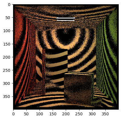
Rainbow visualization

We show three examples:

• Rainbow fusion

• Sparse fusion

• Peak time fusion

All three are based on the same principle: for each pixel, find the time where it reaches its maximum value. Then consider we have a video that is 100 frames long. Using modulo = 20, min_modulo = 0 and max_modulo = 5 means that a pixel will have color only if min_modulo <= frame_max % modulo <= max_modulo.

The way to control this is:

• The bigger the modulo is, the larger the stripes that appear on the image will be

• The bigger the difference between min_modulo and max_modulo, the more pixels that will be painted with color.

rainbow_vis = mitr.vis.rainbow_visualization(
    data_steady,
    data_transient,
    mode='rainbow_fusion',
    modulo=20,
    min_modulo=0,
    max_modulo=5,
    max_time_bins=200)

import matplotlib.pyplot as plt
plt.imshow(rainbow_vis)
plt.show()

rainbow_vis = mitr.vis.rainbow_visualization(
    data_steady,
    data_transient,
    mode='sparse_fusion',
    modulo=10,
    min_modulo=0,
    max_modulo=3,
    max_time_bins=200,
    scale_fusion=0.8)

import matplotlib.pyplot as plt
plt.imshow(rainbow_vis / np.max(rainbow_vis))
plt.show()

rainbow_vis = mitr.vis.rainbow_visualization(
    data_steady,
    data_transient,
    mode='peak_time_fusion',
    modulo=7,
    min_modulo=0,
    max_modulo=1,
    max_time_bins=200,
    scale_fusion=2)

import matplotlib.pyplot as plt
plt.imshow(rainbow_vis)
plt.show()